Hands-on Exercise 4

Author

Lim Li Ying

Visual Statistical Analysis with ggstatsplot

Getting Started

Installing and loading R packages

In this exercise, other than tidyverse, ggstatsplot will also be used. ggstatsplot is an extension of the ggplot2 package and allows details from statistical tests to be added to the information-rich plots.

Click to show/hide the code

pacman::p_load(tidyverse, ggstatsplot)

Loading the data

Click to show/hide the code

exam_data <- read_csv("data/Exam_data.csv")

Rows: 322 Columns: 7
── Column specification ────────────────────────────────────────────────────────
Delimiter: ","
chr (4): ID, CLASS, GENDER, RACE
dbl (3): ENGLISH, MATHS, SCIENCE

ℹ Use `spec()` to retrieve the full column specification for this data.
ℹ Specify the column types or set `show_col_types = FALSE` to quiet this message.

Click to show/hide the code

exam_data

# A tibble: 322 × 7
   ID         CLASS GENDER RACE    ENGLISH MATHS SCIENCE
   <chr>      <chr> <chr>  <chr>     <dbl> <dbl>   <dbl>
 1 Student321 3I    Male   Malay        21     9      15
 2 Student305 3I    Female Malay        24    22      16
 3 Student289 3H    Male   Chinese      26    16      16
 4 Student227 3F    Male   Chinese      27    77      31
 5 Student318 3I    Male   Malay        27    11      25
 6 Student306 3I    Female Malay        31    16      16
 7 Student313 3I    Male   Chinese      31    21      25
 8 Student316 3I    Male   Malay        31    18      27
 9 Student312 3I    Male   Malay        33    19      15
10 Student297 3H    Male   Indian       34    49      37
# ℹ 312 more rows

One-sample test using `gghistostats()`

The code chunk below uses gghistostats() to create a visual of a one-sample test on English scores.

Click to show/hide the code

set.seed(1234)

gghistostats(
  data = exam_data,
  x = ENGLISH,
  type = "bayes",
  test.value = 60,
  xlab = "English scores"
)

Note

Set seed is important especially when doing variance statistics in order to ensure reproducibility.

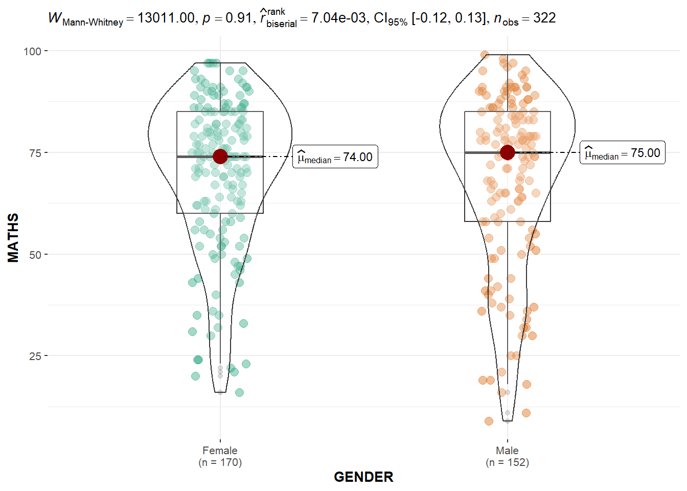
Two-sample mean test using `ggbetweenstats()`

The code chunk below uses ggbetweenstats() to create a visual of a two-sample mean test of Maths scores by gender.

Click to show/hide the code

ggbetweenstats(
  data = exam_data,
  x = GENDER,
  y = MATHS,
  type = "np",
  messages = FALSE
)

Note

There are 4 types of statistical approach:

p <- parametric
np <- nonparametric
r <- robust
b <- bayes

Oneway ANOVA test using `ggbetweenstats()`

The code chunk below uses ggbetweenstats() to create a visual of a oneway ANOVA test of English scores by race.

Click to show/hide the code

ggbetweenstats(
  data = exam_data,
  x = RACE,
  y = ENGLISH,
  type = "p",
  mean.ci = TRUE,
  pairwise.comparisons = TRUE,
  pairwise.display = "s",
  p.adjust.method = "fdr",
  messages = FALSE
)

Note

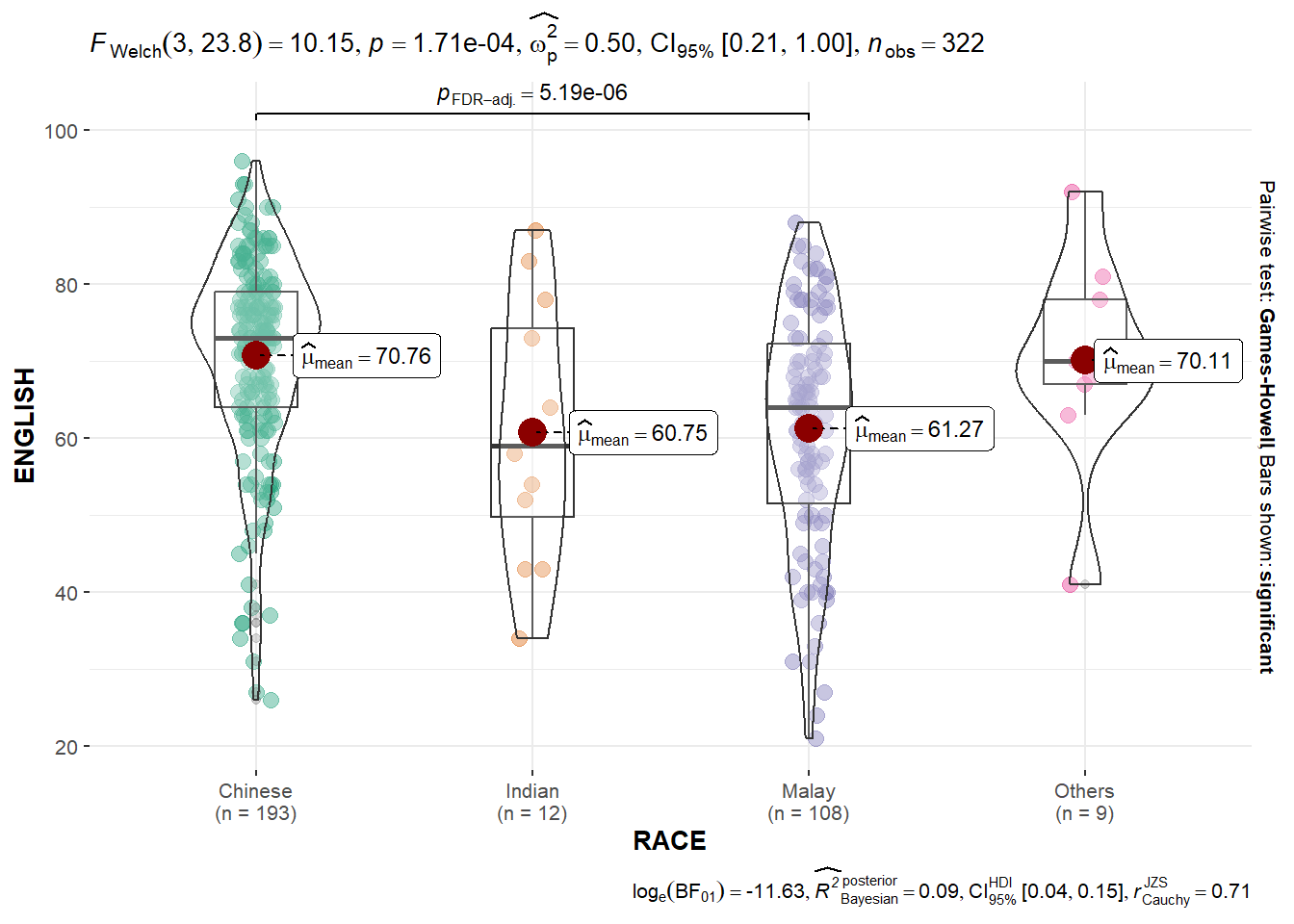
For pairwise display,

s <- displays only significant pairwise comparisons
ns <- displays only non-significant pairwise comparisons
all <- displays all pairwise comparisons

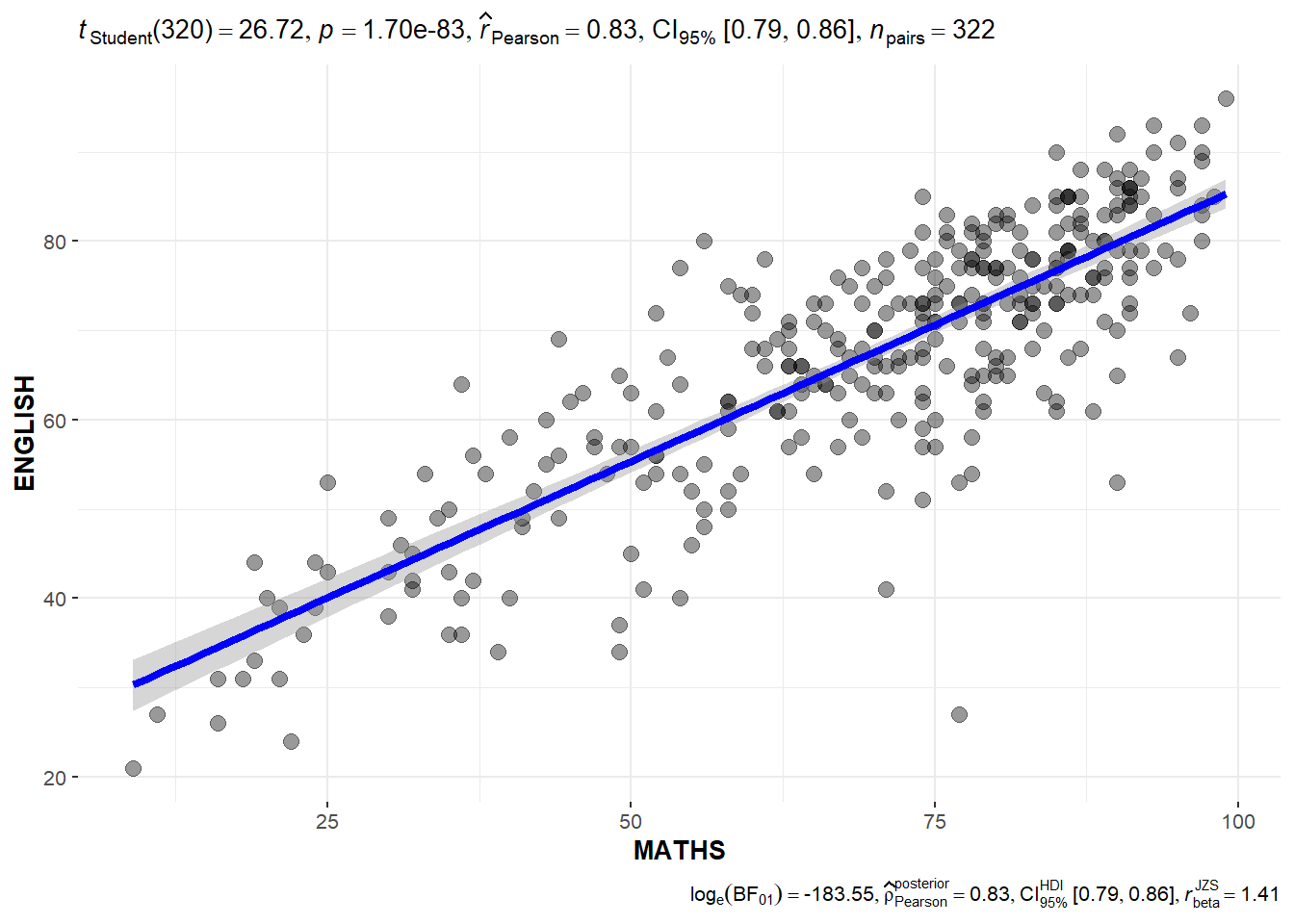
Significant test of correlation using `ggscatterstats()`

The code chunk below uses ggscatterstats() to create a visual of a Significant Test of Correlation between Maths and English scores.

Click to show/hide the code

ggscatterstats(
  data = exam_data,
  x = MATHS,
  y = ENGLISH,
  marginal = FALSE
)

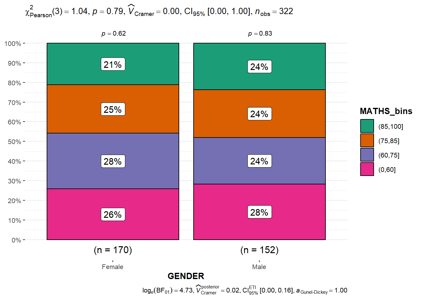
Significant test of association (dependence) using `ggbarstats()`

Firstly, the Maths scores are binned into 4 groups using cut().

Click to show/hide the code

exam_data1 <- exam_data %>%
  mutate(MATHS_bins =
  cut(MATHS, breaks = c(0,60,75,85,100))
)

The code chunk below uses ggbarstats() to create a visual of a Significant Test of Association between Maths scores and gender.

Click to show/hide the code

ggbarstats(
  data = exam_data1,
  x = MATHS_bins,
  y = GENDER
)

Visualizing Models

Getting Started

Installing and loading R packages

The code chunk below shows the R packages to be installed and loaded into the R environment for this exercise.

Click to show/hide the code

pacman::p_load(readxl, performance, parameters, see)

Loading the data

To import the excel worksheet ToyotaCorolla.xls, read_xls() of the readxl package is used, as seen in the code chunk below.

Click to show/hide the code

car_resale <- read_xls("data/ToyotaCorolla.xls")
car_resale

# A tibble: 1,436 × 38
      Id Model    Price Age_08_04 Mfg_Month Mfg_Year     KM Quarterly_Tax Weight
   <dbl> <chr>    <dbl>     <dbl>     <dbl>    <dbl>  <dbl>         <dbl>  <dbl>
 1    81 TOYOTA … 18950        25         8     2002  20019           100   1180
 2     1 TOYOTA … 13500        23        10     2002  46986           210   1165
 3     2 TOYOTA … 13750        23        10     2002  72937           210   1165
 4     3  TOYOTA… 13950        24         9     2002  41711           210   1165
 5     4 TOYOTA … 14950        26         7     2002  48000           210   1165
 6     5 TOYOTA … 13750        30         3     2002  38500           210   1170
 7     6 TOYOTA … 12950        32         1     2002  61000           210   1170
 8     7  TOYOTA… 16900        27         6     2002  94612           210   1245
 9     8 TOYOTA … 18600        30         3     2002  75889           210   1245
10    44 TOYOTA … 16950        27         6     2002 110404           234   1255
# ℹ 1,426 more rows
# ℹ 29 more variables: Guarantee_Period <dbl>, HP_Bin <chr>, CC_bin <chr>,
#   Doors <dbl>, Gears <dbl>, Cylinders <dbl>, Fuel_Type <chr>, Color <chr>,
#   Met_Color <dbl>, Automatic <dbl>, Mfr_Guarantee <dbl>,
#   BOVAG_Guarantee <dbl>, ABS <dbl>, Airbag_1 <dbl>, Airbag_2 <dbl>,
#   Airco <dbl>, Automatic_airco <dbl>, Boardcomputer <dbl>, CD_Player <dbl>,
#   Central_Lock <dbl>, Powered_Windows <dbl>, Power_Steering <dbl>, …

Multiple linear regression modelling using `lm()`

The following code chunk is uses lm() to build a multiple linear regression model.

Click to show/hide the code

model <- lm(Price ~ Age_08_04 + Mfg_Year + KM + 
              Weight + Guarantee_Period, data = car_resale)
model


Call:
lm(formula = Price ~ Age_08_04 + Mfg_Year + KM + Weight + Guarantee_Period, 
    data = car_resale)

Coefficients:
     (Intercept)         Age_08_04          Mfg_Year                KM  
      -2.637e+06        -1.409e+01         1.315e+03        -2.323e-02  
          Weight  Guarantee_Period  
       1.903e+01         2.770e+01

Model diagnostics: checking for multicollinearity

Multicollinearity can be checked using check_collinearity() of the performance package, as seen in the code chunk below.

Click to show/hide the code

check_collinearity(model)

# Check for Multicollinearity

Low Correlation

             Term  VIF     VIF 95% CI Increased SE Tolerance Tolerance 95% CI
               KM 1.46 [ 1.37,  1.57]         1.21      0.68     [0.64, 0.73]
           Weight 1.41 [ 1.32,  1.51]         1.19      0.71     [0.66, 0.76]
 Guarantee_Period 1.04 [ 1.01,  1.17]         1.02      0.97     [0.86, 0.99]

High Correlation

      Term   VIF     VIF 95% CI Increased SE Tolerance Tolerance 95% CI
 Age_08_04 31.07 [28.08, 34.38]         5.57      0.03     [0.03, 0.04]
  Mfg_Year 31.16 [28.16, 34.48]         5.58      0.03     [0.03, 0.04]

Note

Variables with a Variance Inflation Factor (VIF) score of >10 are considered to be highly correlated. In this case, age and manufacturing year have high correlation. Therefore one of the variables will need to be removed from subsequent models.

Click to show/hide the code

check_c <- check_collinearity(model)
plot(check_c)

Variable `Component` is not in your data frame :/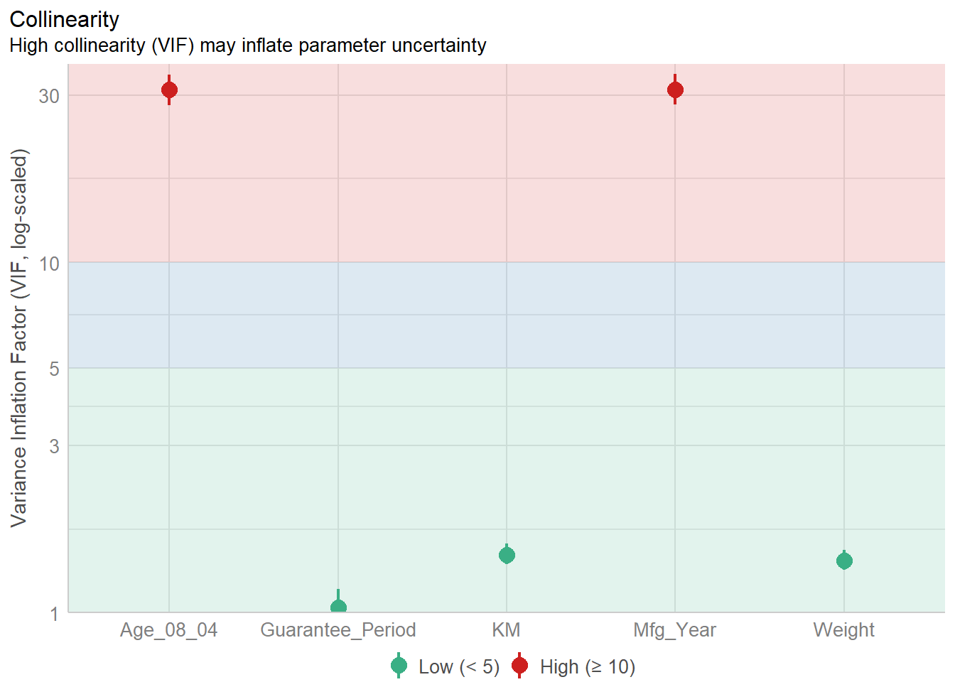

Model diagnostic: checking normality assumption

The normality assumption can be checked using check_normality() of the performance package, as seen in the code chunk below.

Click to show/hide the code

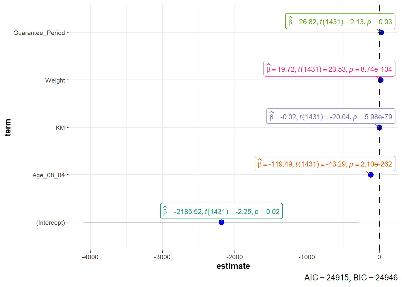
# build another model after removing "Mfg_Year"
model1 <- lm(Price ~ Age_08_04 + KM + 
              Weight + Guarantee_Period, data = car_resale)
check_n <- check_normality(model1)
plot(check_n)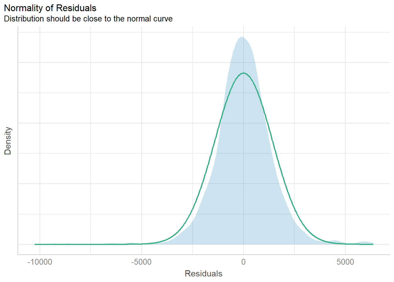

Model diagnostic: checking for homogeneity of variances

Homogeneity of variances can be checked using check_heteroscedasticity() of the performance package, as seen in the code chunk below.

Click to show/hide the code

check_h <- check_heteroscedasticity(model1)
plot(check_h)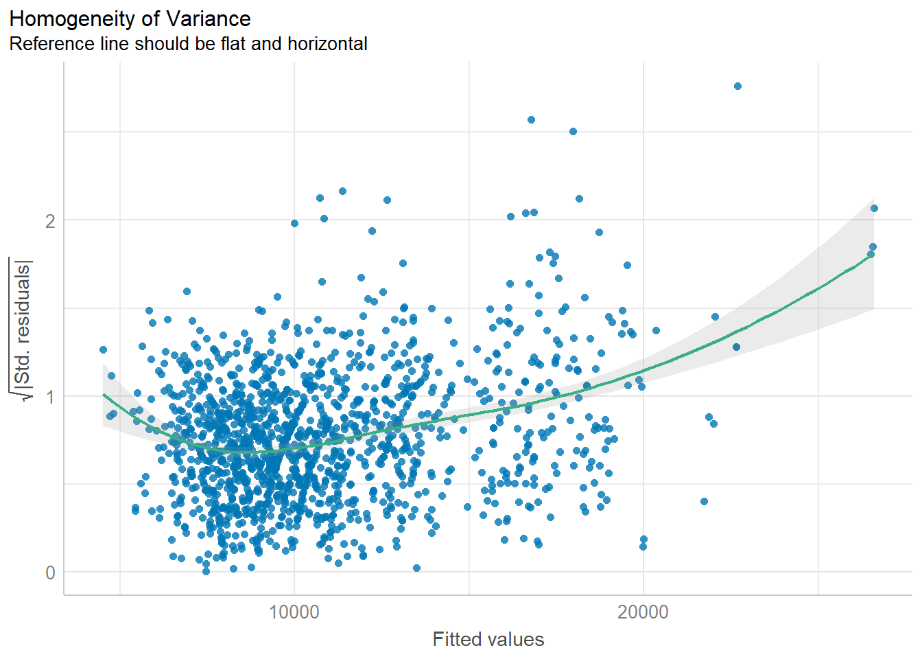

Model diagnostic: complete check

We can also perform a complete check using check_model().

Click to show/hide the code

check_model(model1)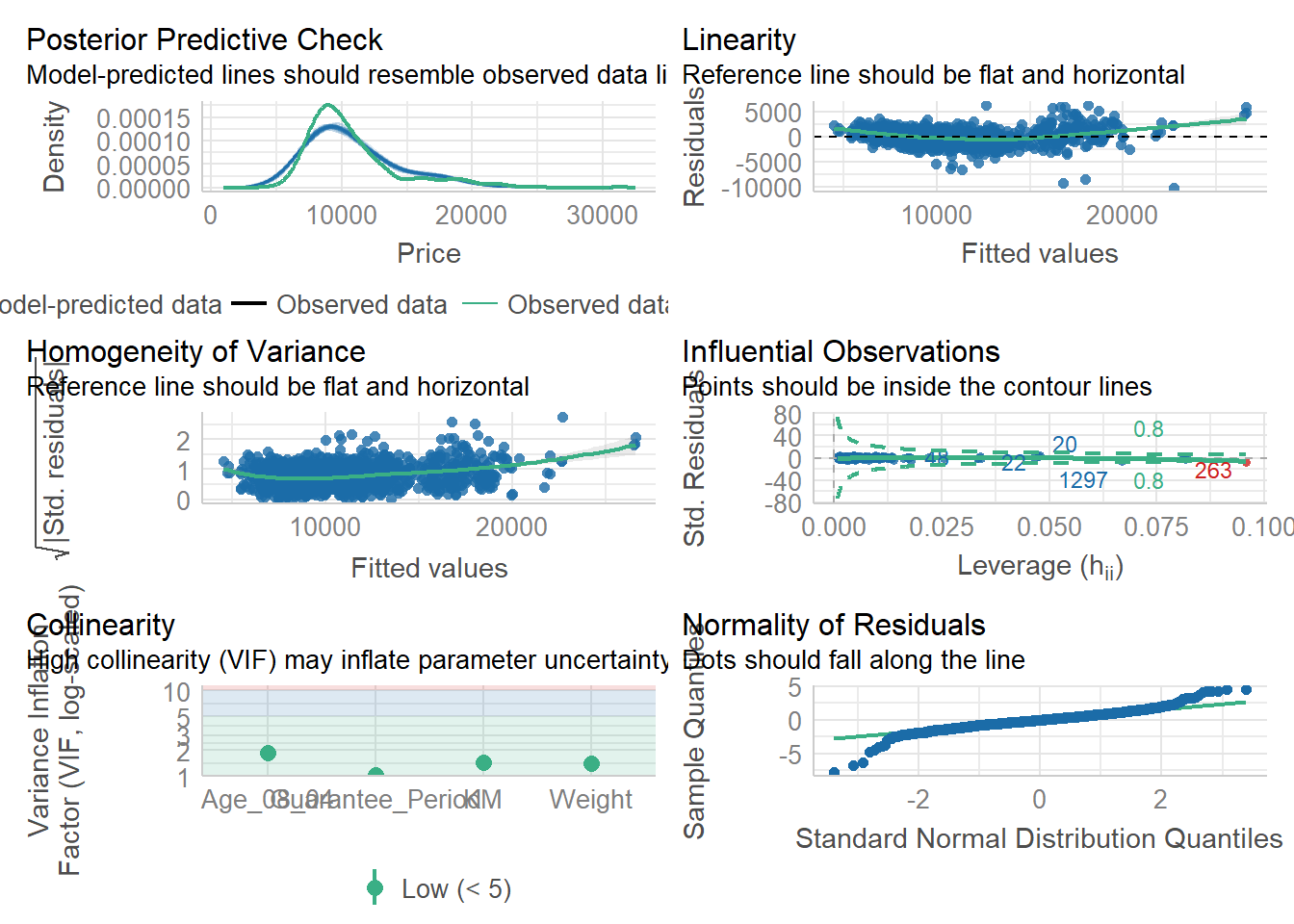

Visualizing regression parameters using see

Click to show/hide the code

plot(parameters(model1))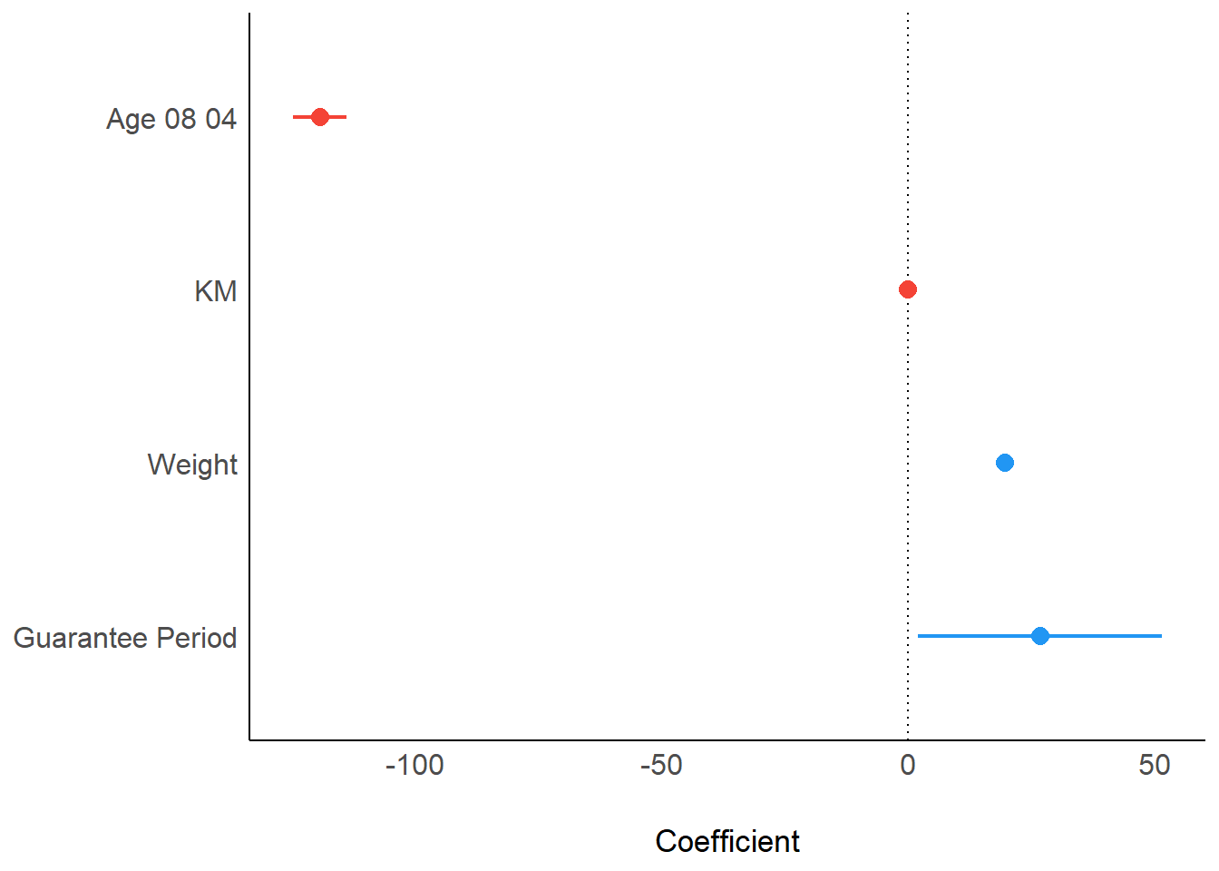

Visualizing regression parameters using `ggcoefstats()`

Click to show/hide the code

ggcoefstats(model1,
            output = "plot")

Visual Statistical Analysis with ggstatsplot

Getting Started

Installing and loading R packages

Loading the data

One-sample test using gghistostats()

Two-sample mean test using ggbetweenstats()

Oneway ANOVA test using ggbetweenstats()

Significant test of correlation using ggscatterstats()

Significant test of association (dependence) using ggbarstats()

Visualizing Models

Getting Started

Installing and loading R packages

Loading the data

Multiple linear regression modelling using lm()

Model diagnostics: checking for multicollinearity

Model diagnostic: checking normality assumption

Model diagnostic: checking for homogeneity of variances

Model diagnostic: complete check

Visualizing regression parameters using see

Visualizing regression parameters using ggcoefstats()

One-sample test using `gghistostats()`

Two-sample mean test using `ggbetweenstats()`

Oneway ANOVA test using `ggbetweenstats()`

Significant test of correlation using `ggscatterstats()`

Significant test of association (dependence) using `ggbarstats()`

Multiple linear regression modelling using `lm()`

Visualizing regression parameters using `ggcoefstats()`